MIR: using different interpolations

This example compares different interpolation methods using the mir backend.

To make this notebook work earthkit-data and earthkit-plots have to be installed. The data will be represented as an earthkit-data GRIB FieldList.

Regridding

We perform the regridding with the regrid() method.

from earthkit.regrid import regrid
import earthkit.data as ekd

# Get octahedral reduced Gaussian GRIB data containing two fields.
ds = ekd.from_source("sample", "O32_t2.grib2")

# the target grid is a global 1x1 degree regular latitude-longitude grid
grid = {"grid": [1,1]}

# Regrid the fieldlist using various interpolations and
# gather results in a dict
res = {}
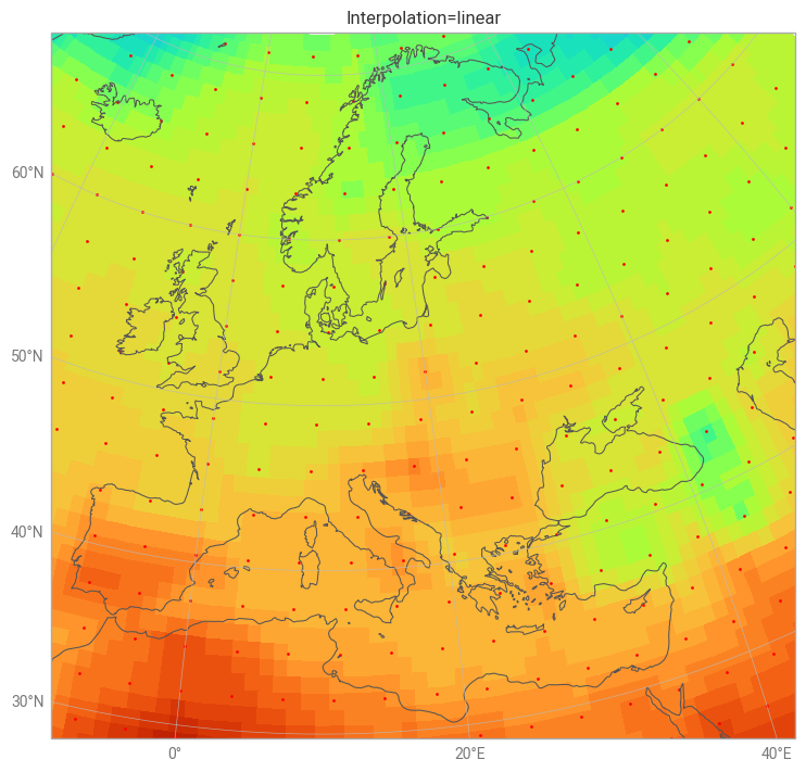
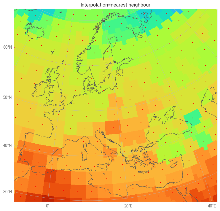
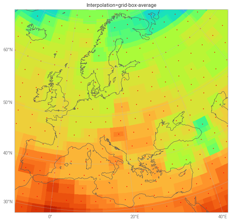
for i_type in ["linear", "nearest-neighbour", "grid-box-average"]:
    res[i_type] = regrid(ds, grid=grid, interpolation=i_type)

Plotting the results

We use earthkit-plots to visualise the results together with the locations of the original (O32) gridpoints.

import earthkit.plots as ekp

for i_type, ds_res in res.items():
    chart = ekp.Map(domain=["Europe"])
    # we only plot the first field from the result
    chart.grid_cells(ds_res[0], units="celsius", auto_style=True)
    # plot the original grid points
    chart.grid_points(ds[0])
    chart.title(f"interpolation={i_type}")
    chart.coastlines()
    chart.gridlines()
    chart.show()